For ALL octahedral complexes, except high spin d5, simple CFT would predict that only 1 band should appear in the electronic spectrum and that the energy of this band should correspond to the absorption of energy equivalent to Δ. In practice, ignoring spin-forbidden lines, this is only observed for those ions with D free ion ground terms i.e., d1, d9 as well as d4, d6.
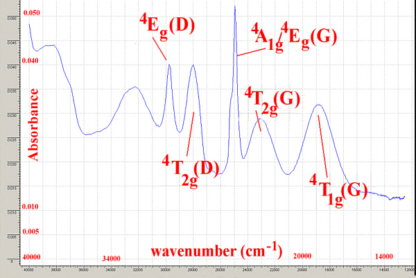
The observation of 2 or 3 peaks in the electronic spectra of d2, d3, d7 and d8 high spin octahedral complexes requires further treatment involving electron-electron interactions. Using the Russell-Saunders (LS) coupling scheme, these free ion configurations give rise to F free ion ground states which in octahedral and tetrahedral fields are split into terms designated by the symbols A2(g), T2(g) and T1(g).
To derive the energies of these terms and the transition energies between them is beyond the needs of introductory level courses and is not covered in general textbooks[10,11]. A listing of some of them is given here as an Appendix. What is necessary is an understanding of how to use the diagrams, created to display the energy levels, in the interpretation of spectra.
In the laboratory component of the course we will measure the absorption spectra of some typical chromium(III) complexes and calculate the spectrochemical splitting factor, Δ. This corresponds to the energy found from the first transition below and as shown in Table 1 is generally between 15,000 cm-1 (for weak field complexes) and 27,000 cm-1 (for strong field complexes).
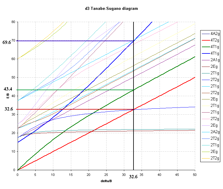
For the d3 octahedral case, 3 peaks can be predicted and these would correspond to the following transitions and energies:
where C.I. is the configuration interaction arising from the "non-crossing rule".
|
Complex
|
ν1
|
ν2
|
ν3
|
ν2/ ν1
|
ν1/ ν2
|
Δ/B
|
Ref
|
| Cr3+ in emerald |
16260
|
23700
|
37740
|
1.46
|
0.686
|
20.4
|
13 |
| K2NaCrF6 |
16050
|
23260
|
35460
|
1.45
|
0.690
|
21.4
|
13 |
| [Cr(H2O)6]3+ |
17000
|
24000
|
37500
|
1.41
|
0.708
|
24.5
|
This work |
| Chrome alum |
17400
|
24500
|
37800
|
1.36
|
0.710
|
29.2
|
4 |
| [Cr(C2O4)3]3- |
17544
|
23866
|
? |
1.37
|
0.735
|
28.0
|
This work |
| [Cr(NCS)6]3- |
17800
|
23800
|
? |
1.34
|
0.748
|
31.1
|
4 |
| [Cr(acac)3] |
17860
|
23800
|
? |
1.33
|
0.752
|
31.5
|
This work |
| [Cr(NH3)6]3+ |
21550
|
28500
|
? |
1.32
|
0.756
|
32.6
|
4 |
| [Cr(en)3]3+ |
21600
|
28500
|
? |
1.32
|
0.758
|
33.0
|
4 |
| [Cr(CN)6]3- |
26700
|
32200
|
? |
1.21
|
0.829
|
52.4
|
4 |
For octahedral Ni(II) complexes the transitions would be:
where C.I. again is the configuration interaction and as before the first transition corresponds exactly to Δ.
For M(II) the size of Δ is much less than for M(III) and typical values for Ni(II) are 6500 to 13000 cm-1 as shown in Table 2.
|
Complex
|
ν1
|
ν2
|
ν3
|
ν1
|
ν1/ ν2
|
Δ/B
|
Ref
|
| NiBr2 |
6800
|
11800
|
20600
|
1.74
|
0.576
|
5
|
13 |
| [Ni(H2O)6]2+ |
8500
|
13800
|
25300
|
1.62
|
0.616
|
11.6
|
13 |
| [Ni(gly)3]- |
10100
|
16600
|
27600
|
1.64
|
0.608
|
10.6
|
13 |
| [Ni(NH3)6]2+ |
10750
|
17500
|
28200
|
1.63
|
0.614
|
11.2
|
13 |
| [Ni(en)3]2+ |
11200
|
18350
|
29000
|
1.64
|
0.610
|
10.6
|
3 |
| [Ni(bipy)3]2+ |
12650
|
19200
|
? |
1.52
|
0.659
|
17
|
3 |
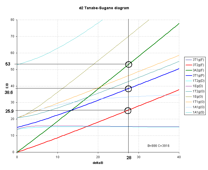
For d2 octahedral complexes, few examples have been published. One such is V3+ doped in Al2O3 where the vanadium ion is generally regarded as octahedral, Table 3.
|
Complex
|
ν1
|
ν2
|
ν3
|
ν2/ ν1
|
ν1/ν2
|
Δ/B
|
Ref
|
| V3+ in Al2O3 |
17400
|
25200
|
34500
|
1.448
|
0.6906
|
30.90
|
13 |
| [VCl3(MeCN)3] |
14400
|
21400
|
?
|
1.486
|
0.6729
|
28.68
|
4 |
| K3[VF6] |
14800
|
23250
|
?
|
1.571
|
0.6365
|
24.78
|
4 |
Interpretation of the spectrum highlights the difficulty of using the right-hand side of the Orgel diagram as previously noted. For d2 cases where none of the transitions correspond exactly to Δ often only 2 of the 3 transitions are clearly observed and hence the calculations will have three unknowns (Δ, B and C.I.) but only 2 energies to use in the the analysis.
The first transition can be unambiguously assigned as:
3T2g ← 3T1g ĀĀĀĀĀĀĀĀĀ transition energy = 4/5 * Δ + C.I.But, depending on the size of the ligand field ( Δ) the second transition may be due to:
3A2g ← 3T1g ĀĀĀĀĀĀĀĀĀ transition energy = 9/5 * Δ + C.I.for a weak field or
3T1g(P) ← 3T1g ĀĀĀĀĀ transition energy = 3/5 * Δ + 15B' + 2 * C.I.for a strong field.
The transition energies of these terms are clearly different and it is often necessary to calculate (or estimate) values of B, Δ and C.I. for both arrangements and then evaluate the answers to see which fits better.
The difference between the 3A2g and the 3T2g (F) lines should give Δ. In this case Δ is equal to either:Solving the equations like this for the three unknowns can ONLY be done if the three transitions are observed. When only two transitions are observed, a series of equations[14] have been determined that can be used to calculate both B and Δ. This approach still requires some evaluation of the numbers to ensure a valid fit. For this reason, Tanabe-Sugano diagrams become a better method for interpreting spectra of d2 octahedral complexes.
The Nephelauxetic Series is given by:
F- < H2O < urea < NH3 < en ~ C2O42- < NCS- < Cl- ~ CN- < Br- < S2- ~ I-This series is consistent with fluoride complexes being the most ionic and giving a small reduction in B while covalently bonded ligands such as I- give a large reduction of B.
As an example of a Cr(III) complex, using the observed peaks
found for [Cr(NH3)6]3+ in Table
1 above, namely ν1 = 21550 cm-1 and ν2 = 28500 cm-1 the
ratio of ν2/ν1 = 1.32.
The value of Δ is obtained directly from the first transition
so Δ/B' is equal to ν1/B' and finding B' is now relatively
straightforward since from the first transition energy of 21,550
cm-1 and the value of Δ/B' (ν1/B') of 32.6 we get:
B' = 21,550/ 32.6 or B' = 661 cm-1
The third peak can then be predicted to occur at 69.64 * 661 = 46030
cm-1 or 217 nm (well in the UV region and probably
hidden by charge transfer or solvent bands).
It is important to remember that for spectra recorded in solution the width of the peaks may be as large as 1-2000 cm-1 so as long as it is possible to unambiguously assign peaks, the techniques are valuable.
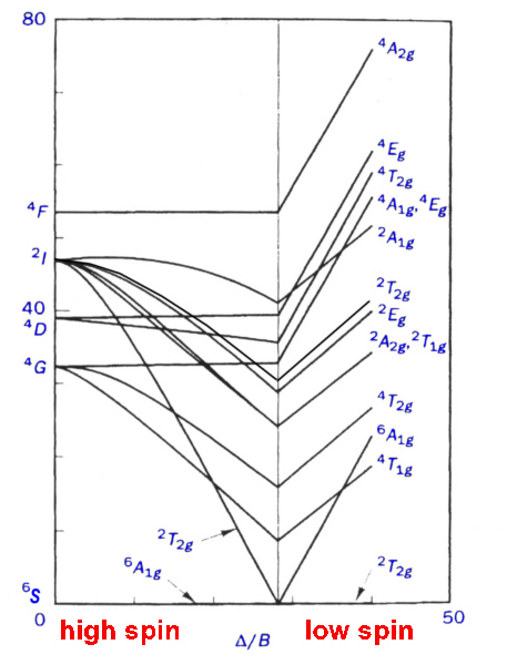
To overcome the problem of small diagrams found in textbooks, it was decided to generate our own Tanabe-Sugano diagrams using spreadsheets. This was done, using the transition energies given in the Appendix, for the spin-allowed transitions and using CAMMAG to generate the energies of the spin-forbidden transitions.
Even so, the method of finding the correct X-intercept is somewhat tedious and time-consuming and a different approach was devised using JAVA applets.
The JAVA applets display the transitions and when the user clicks on any region of the graph then the values of ν2/ ν1 and ν3/ν1 are displayed. In addition, the values of Δ/B and the Y-intercepts are given as well. This simplifies the process of determining the best fit for Δ/B.
The expected ranges for the ratio of ν2/ν1 are:
These ratios show the need for a certain degree of precision in attempting to analyse the spectra, especially for d7 and d8. It has been suggested that instead of using ν2/ ν1 that any two ratios can be used and graphs of these plots were produced by Lever in the 1960's[11]. Once again though the published diagrams are rather small and so the spreadsheets above contain these charts which can be printed in larger scale. The slopes of the various ratio lines vary greatly and it is useful to examine the region of interest first before deciding on which set of lines should be used for analysis. If only 2 peaks are observed then this is not an option.
For the spin-allowed diagrams:Further information for use in laboratory classes is available and some example calculations are available as well.
Transitions calculated for spin-allowed terms in the Tanabe-Sugano diagrams.
Octahedral d3 (e.g. Chromium(III) ).
4T2g ← 4A2g , ν1/B= Δ/B
4T1g(F) ← 4A2g, ν2/B= ½{15 + 3( Δ/B) - √(225 - 18(Δ/B) + ( Δ/B)2 ) }
4T1g(P) ← 4A2g, ν3/B= ½{15 + 3( Δ/B) + √(225 - 18(Δ/B) + ( Δ/B)2 ) }
from this, the ratio ν2/ν1 would become:
½{15 + 3( Δ/B) - √(225 - 18(Δ/B) + ( Δ/B)2 ) } / Δ/B
and the range of Δ/B required is from ~15 to ~55
Octahedral d8 (e.g. Nickel(II) ).
3T2g ← 3A2g, ν1/B= Δ/B
3T1g(F) ← 3A2g, ν2/B= ½{15 + 3(Δ/B) - √(225 - 18(Δ/B) + ( Δ/B)2 ) }
3T1g(P) ← 3A2g, ν3/B= ½{15 + 3(Δ/B) + √(225 - 18(Δ/B) + ( Δ/B)2 ) }
from this the ratio ν2/ν1 would become:
½{15 + 3( Δ/B) - √(225 - 18(Δ/B) + ( Δ/B)2 ) } / Δ/B
and the range of Δ/B required is from ~5 to ~17
Octahedral d2 (e.g. Vanadium(III) ).
3T2g ← 3T1g , ν1/B= ½{(Δ/B) - 15 + √(225 + 18(Δ/B) + ( Δ/B)2 ) }
3T1g(P) ← 3T1g, ν2/B= √(225 + 18(Δ/B) + (Δ/B)2 )
3A2g ← 3T1g, ν3/B= ½{ 3 (Δ/B) -15 + √(225 + 18(Δ/B) + ( Δ/B)2 ) }
from this the ratio ν2/ν1 would become:
√(225 + 18(Δ/B) + ( Δ/B)2 ) / ½{( Δ/B) - 15 + √(225 + 18(Δ/B) + ( Δ/B)2 ) }
and the range of Δ/B required is from ~15 to ~35
Tetrahedral d7 (e.g. Cobalt(II) ).
4T2 ← 4A2, ν1/B= Δ/B
4T1 (F) ← 4A2, ν2/B= ½{15 + 3(Δ/B) - √(225 - 18(Δ/B) + ( Δ/B)2 ) }
4T1 (P) ← 4A2, ν3/B= ½{15 + 3(Δ/B) + √(225 - 18(Δ/B) + ( Δ/B)2 ) }
from this the ratio ν2/ν1 would become:
½{15 + 3(Δ/B) - √(225 - 18( Δ/B) + ( Δ/B)2 ) } / Δ/B
and the range of Δ/B required is from ~3 to ~8.
Thanks are due to Christopher Muir, for help with developing the JAVA applets.
 Return to Chemistry, UWI-Mona,
Home Page
Return to Chemistry, UWI-Mona,
Home Page
Copyright © 1999-2011 by Robert John Lancashire, all rights reserved.
Created and maintained by Prof. Robert J. Lancashire